semEff can be used to predict values for different types
of effects in an SEM. For example, we may be interested in the
predictions of an indirect effect of a variable vs. its direct effect,
or we may simply wish to predict the total (combined) effect. Here we’ll
use simulated
data from Shipley (2009) on tree growth and survival for
a single tree species to predict and plot a direct vs. indirect
effect.
Let’s preview the data (n = 1900):
| site | tree | lat | year | Date | DD | Growth | Survival | Live |
|---|---|---|---|---|---|---|---|---|
| 1 | 1 | 40.38063 | 1970 | 115.4956 | 160.5703 | 61.36852 | 0.9996238 | 1 |
| 1 | 2 | 40.38063 | 1970 | 118.4959 | 158.9896 | 43.77182 | 0.8433521 | 1 |
| 1 | 3 | 40.38063 | 1970 | 115.8836 | 159.9262 | 44.74663 | 0.9441110 | 1 |
| 1 | 4 | 40.38063 | 1970 | 110.9889 | 161.1282 | 48.20004 | 0.9568525 | 1 |
| 1 | 5 | 40.38063 | 1970 | 120.9946 | 157.3778 | 50.02237 | 0.9759584 | 1 |
| 1 | 1 | 40.38063 | 1972 | 114.2315 | 160.6120 | 56.29615 | 0.9983398 | 1 |
Tree measurements are taken for five individuals of the same species
at 20 different sites every two years from 1970 to 2006 (repeated
measures). The hypothesised SEM from Shipley (2009) tests the indirect effect of
site latitude on tree survival (0/1), via degree days to bud burst, date
of first bud burst, and tree growth. This can be fit as a series of
linear and generalised linear mixed models using the lme4
package:
shipley.sem <- list(
  DD = lme4::lmer(DD ~ lat + (1 | site) + (1 | tree), data = shipley),
  Date = lme4::lmer(Date ~ DD + (1 | site) + (1 | tree), data = shipley),
  Growth = lme4::lmer(Growth ~ Date + (1 | site) + (1 | tree), data = shipley),
  Live = lme4::glmer(Live ~ Growth + (1 | site) + (1 | tree), data = shipley,
                     family = binomial)
)
We can bootstrap estimates for these models:
shipley.sem.boot <- bootEff(shipley.sem, R = 1000, seed = 13, ran.eff = "site")And use the bootstrap samples to calculate effects and confidence intervals:
(shipley.sem.eff <- semEff(shipley.sem.boot))
#>
#> Piecewise SEM with:
#>   * 1 exogenous vs. 4 endogenous variable(s)
#>   * 4 direct vs. 6 indirect effect(s)
#>
#> Variables:
#>           Category   Predictor Mediator Response   Dir. Eff. Ind. Eff.
#>           --------   --------- -------- --------   --------- ---------
#>  lat    | Exog.    |     x        -        -     |         -         - |
#>  DD     | Endog.   |     x        x        x     |         1         0 |
#>  Date   | Endog.   |     x        x        x     |         1         1 |
#>  Growth | Endog.   |     x        x        x     |         1         2 |
#>  Live   | Endog.   |     -        -        x     |         1         3 |
#>
#> Use summary() for effects and confidence intervals for endogenous variables.
#> See ?getEff() for extracting (unformatted) effects.
For this example, let’s compare the direct effects of Date (Julian date of first bud burst) vs. the indirect effects of DD (cumulative degree days to first bud burst, °C) on tree Growth (increase in stem diameter, mm):
summary(shipley.sem.eff, "Growth")
#>
#> SEM direct, summed indirect, total, and mediator effects:
#>
#> Response 'Growth' (3/4):
#>                    Effect     Bias   Std. Err.   Lower CI Upper CI
#>                    ------   ------   ---------   -------- --------
#>  DIRECT:    Date |  0.382 |  0.011 |     0.058 |    0.293    0.515 | *
#>                  |        |        |           |                   |
#>  INDIRECT:  lat  |  0.165 |  0.001 |     0.048 |    0.086    0.281 | *
#>             DD   | -0.240 | -0.007 |     0.042 |   -0.344   -0.181 | *
#>                  |        |        |           |                   |
#>  TOTAL:     lat  |  0.165 |  0.001 |     0.048 |    0.086    0.281 | *
#>             DD   | -0.240 | -0.007 |     0.042 |   -0.344   -0.181 | *
#>             Date |  0.382 |  0.011 |     0.058 |    0.293    0.515 | *
#>                  |        |        |           |                   |
#>  MEDIATORS: DD   |  0.165 |  0.001 |     0.048 |    0.086    0.281 | *
#>             Date | -0.075 | -0.006 |     0.017 |   -0.109   -0.049 | *
We’ll extract the (total) effects of each variable to use for prediction:
tot <- getTotEff(shipley.sem.eff, "Growth")
tot.b <- getTotEff(shipley.sem.eff, "Growth", type = "boot")
Now we can predict values for Growth using predEff().
We’ll need the model object, and we’ll generate 100 values of the
predictors to predict from:
dat <- na.omit(shipley)
mod <- shipley.sem$Growth
fit <- sapply(c("Date", "DD"), function(i) {
  x <- data.frame(seq(min(dat[i]), max(dat[i]), length = 100)); names(x) <- i
  f <- predEff(mod, newdata = x, effects = tot[i], eff.boot = tot.b)
  c(x, f)
}, simplify = FALSE)
OK let’s plot the predictions. We’ll use a custom plotting function
which wraps ggplot2::ggplot():
plotFit <- function(x, y, fit, x.lab = NULL, y.lab = NULL) {
  d <- fit[[1]]
  f <- fit$fit
  ci.l <- fit$ci.lower
  ci.u <- fit$ci.upper
  ggplot () +
    geom_point(aes(x, y)) +
    geom_ribbon(aes(d, ymin = ci.l, ymax = ci.u, alpha = "0.15"), fill = "blue") +
    geom_line(aes(d, f), color = "blue", size = 1) +
    xlab(x.lab) +
    ylab(y.lab) +
    theme_bw() +
    theme(legend.position = "none")
}
Effects of Date (direct):
plotFit(x = dat$Date, y = dat$Growth, fit = fit$Date,
        x.lab = "Julian Date of Bud Burst (direct effect)", y.lab = "Stem Growth (mm)")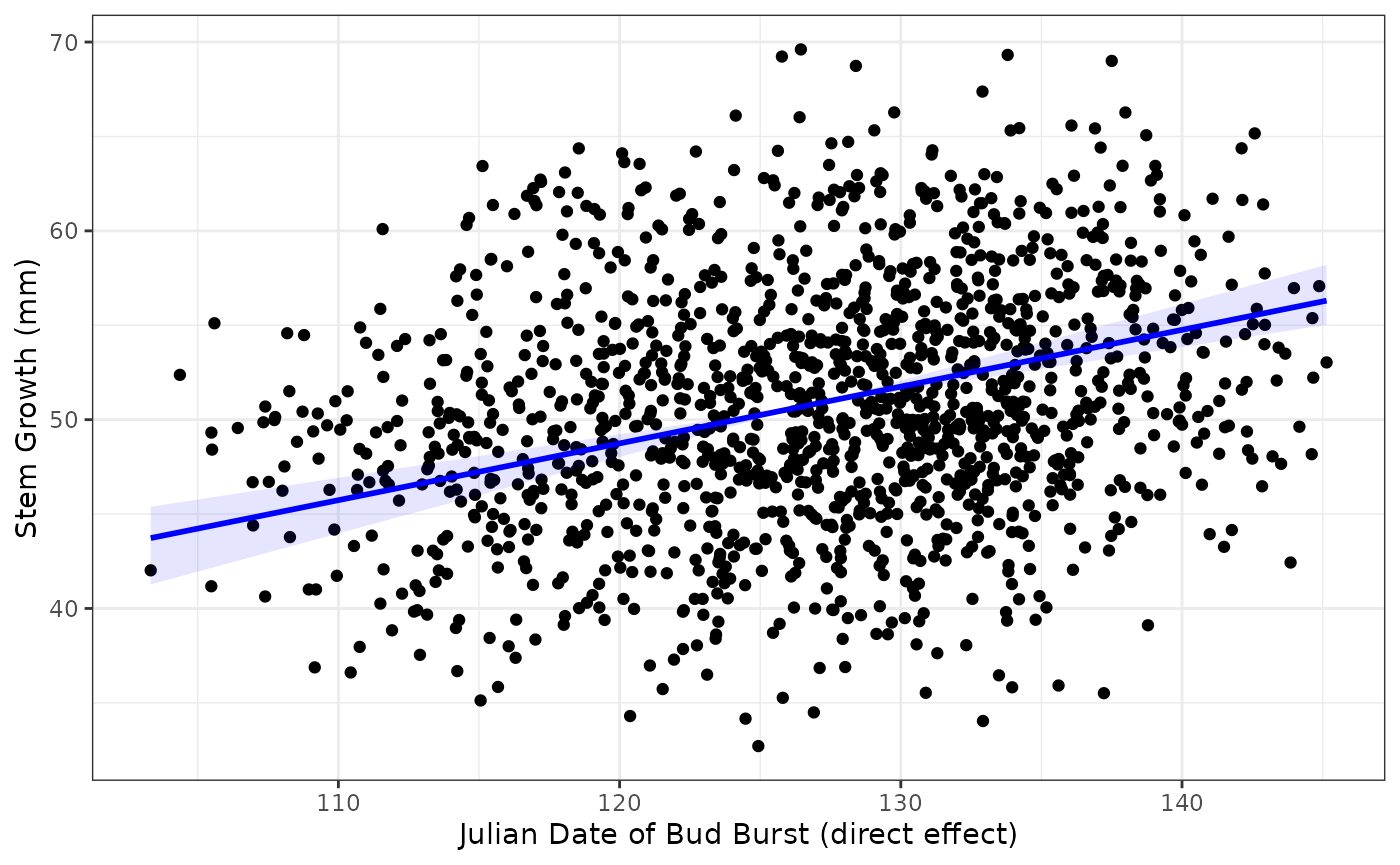
Effects of DD (indirect, via Date):
plotFit(x = dat$DD, y = dat$Growth, fit = fit$DD,
        x.lab = "Degree Days to Bud Burst (indirect effect)", y.lab = "Stem Growth (mm)")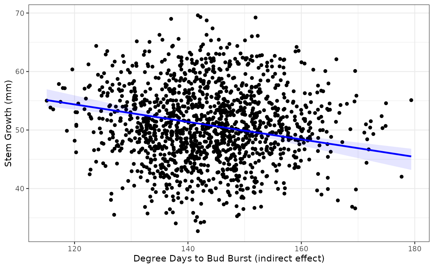
We can see that the effects are in opposite directions: positive for Date (direct) and negative for DD (indirect). This is because trees at higher latitudes require fewer degree days to break buds (cooler climate), break buds later, and grow more in the growing season than trees at lower latitudes. Thus DD negatively affects Growth by reducing the Date to first bud burst. This is just a toy example from the SEM to illustrate contrasting effects of similar magnitude. DD in this case is acting as a proxy for latitude (high DD = low latitude).
It’s also evident from the plots that there is a huge amount of
scatter around the fits. This is due to the random effects (‘site’ and
‘tree’) accounting for most variation in tree growth. We can get a rough
breakdown of this using R-squared, here via R2()
(squared multiple correlation):
c(r2_marg = R2(mod, re.form = NA)[[1]],
  r2_cond = R2(mod)[[1]])
#>    r2_marg    r2_cond
#> 0.04814953 0.79383672
Fixed (‘marginal’) effects account for only about 5% of variation, compared to almost 80% when adding all random effects (‘conditional’). We can also condition on individual random effects, showing that ‘tree’ accounts for most random variation:
c(r2_site = R2(mod, re.form = ~ 1 | site)[[1]],
  r2_tree = R2(mod, re.form = ~ 1 | tree)[[1]])
#>   r2_site   r2_tree
#> 0.3081469 0.6068561